Chapter 1

INTRODUCTION TO DISCRETE EVENT SIMULATION

1.1 Introduction

A dictionary definition of the verb simulate might be some form of words like: to mimic, to take the form of something. In this context it is often used to mean a form of deceit. However in mathematical modelling we use the word to represent the numerical time advance modelling of some real world system.

Computer simulation is a powerful tool that is often applied to the design and analysis of complex systems. Decisions can be made about the system by constructing computer models of it and conducting experiments on the model.

1.2 What is the Purpose of Simulation ?

There are a number of reasons why it may be preferable to carry out experiments on a model rather than directly on the real system:

• The results of the experiment may be unpredictable or dangerous to the system or the personnel operating it.
• Experiments may unacceptably disrupt the operational requirements of the system.
• A new system may require design decisions to be made prior to construction of the system.
• A simulation experiment may be precisely repeated any number of times. In many instances a real dynamic system would not allow precise replication.
• Confidentiality is easier to maintain with a computer simulation where only a few key people would be privy to the results. The results of experimenting with a real system are more open.
• Time scale of the real system may be too long (e.g. evolution of a galaxy), or too short (e.g. impact between vehicles) for convenient experimentation.
• Training.

1.3 Simulation Models

A simulation project involves building a model of the system to be studied. In order to do this we must clearly understand what we mean by a model. Models, for our purpose, fall into three categories:

1. Iconic & physical models. These are physical models usually at a reduced scale. Examples are wooden models of cars or an aircraft wing and the model describes the shape of the object that is being modelled. The purpose of such models is often to investigate the relationship between the shape of the object and the environment in which it will operate. For example, wind tunnel testing.
2. Abstract models. These are mathematical equations. Examples are the equations describing physical laws of nature and scientific laws. These models often describe motion or forces that exist between objects. The purpose of such models is often to investigate what impact there will be on the system as a whole if changes are made to individual elements of the system.
3. Visual models. These are graphical representations. Examples are schematic diagrams of electronic equipment or flow charts that describe the logic of a computer program. The purpose of these models is usually to enable the operating rules and processes of a system to be understood.

Note the recurrence of the words 'describes' and 'purpose' in this list. A model is a description and the form that the model takes is very dependent on the purpose of the model. The purpose of a model is, therefore, an important aspect of model formulation and must be discussed and agreed before a model of the system can be constructed. The purpose may be expressed in the form of statements concerning what decisions are expected to be made as a result of the simulation study. The model is then constructed in a form that will enable the correct decision to be made.

For example, a company may be wishing to expand production of a particular product. To do this they will need to purchase one or more additional machines. There is a choice between a high throughput, high cost machine or a low throughput, low cost machine. The purpose of the simulation may be to ascertain the number of machines of each type that would be needed to achieve target production.

A Flight Simulator is an example of simulation that comes readily to mind. It is used to train novice pilots to fly modern jet aircraft realistically but without the danger to life that could occur flying a real aircraft. Flight simulators also allow experienced pilots to gain experience with unfamiliar aircraft. A flight simulator consists of an exact replica of an aircraft cockpit with all of the controls and meters but without the fuselage, wings, engines or (and perhaps most importantly!) passengers.

The student pilot uses exactly the same controls and sees the same instruments that would be in a real aircraft of that type. However, the outputs from the controls are passed to a computer rather than to the flaps, engines, undercarriage etc. of a real aircraft. The pilot is given the same sort of feedback that would be experienced flying a real aircraft and the instruments would show readings that reflect a real flight. When the computer senses that a pilot has used a control that would make the nose of the aircraft lift then the computer sends signals to motors that lift the nose of the flight simulator. Similarly it can be made to bank to the left and right; engine noise is made to increase and decrease appropriately; and the view from the cockpit changes in response to changes in direction and inclination. Thus the pilot's senses of touch, sight, hearing and physical orientation receive the same sort of stimuli that they would receive flying a real aircraft. The big difference, however, is that if the pilot 'crashes' the simulator nothing is dented (except perhaps the pilot's pride!).

This is one, obvious, benefit of using a simulator instead of a real aircraft for training purposes but there are others, including:

• immediate access to a specific part of the training programme. If you want to practice landing, the simulator doesn't have to take-off first - - the real aircraft does
• changeover time between students is low. A real aircraft would have to be refuelled and perhaps inspected
• fault situations (random or specific) can be programmed into a training session to test the pilots ability to react correctly and in time.

There is a high degree of correspondence, from the pilot's viewpoint, between flying a simulator and flying a real aircraft. And this is exactly the purpose of the flight simulator.

In other situations such a high level of realism is both unnecessary and undesirable. The simulation model should contain sufficient detail for the functionality of the system to be understood but excluding unnecessary complexity that clouds understanding.

1.4 DES simulation paradigms

A major subclass of simulation problems is concerned with the simulation of time varying systems which are controlled by a combination of either physical, chemical, biological or man made laws. Such systems can be categorised by the way in which time is treated in the simulation. The variation in time may be considered continuous in some systems whilst in others the state of the system changes at discrete time intervals. This phenomenon gives rise to two branches of simulation: Discrete Event Simulation and Continuous Simulation. Clearly, models of such systems must also be capable of changing their state in a similar manner.

Continuous simulation problems are essentially based on the solution of time dependent partial differential equations. If the simulation is computer based only finite steps can be incorporated and, hence, small equal time increments are employed to approximate to the real world situation. Typical applications include:

• Development of eco-systems
• Economic forecasting systems
• Thermal balance in nuclear reactors
• Evolution of stellar systems

Discrete simulation examines problems in which the ordering and timing of events is the main focus of interest. In such systems the interest is on on the time at which some activity commences or ceases. For example, in simulating a computer network to estimate the effective system capacity or queue sizes, we may be interested in the start time and duration of job processing rather than details of the signal transmission on the network. In such problems it is not efficient to advance time in small fixed steps but to advance to the time of the next event. Since, in general, events can occur at any time, the time advance is non-uniform and can be alternately large or small. Typical applications include:

• Factory layout and process planning.
• Transport systems.
• Telecommunications networks.
• Office management systems.

Discrete simulation can be further subdivided in terms of the methodology followed. Figure 1 shows the general scheme.

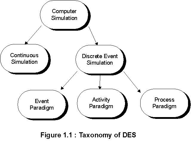
Event	The events and their consequences that influence the progress of the simulation are listed and the simulation is progressed by working through a time based 'event list'.
Activity	For each entry (product, resource etc.) that is involved in the simulation a cycle of activities is drawn up. All entity cycles are then merged into a single activity diagram which forms the basis of the model.
Process	The processes through which the 'key' entities pass is listed as a sequence which forms the basis of the model. The key entities are usually the product being studied and other entities become resources used by the key entities.

The three types are not exclusive and, in general, a study can be formulated in any of the paradigms. Mixed paradigm representations are also possible.

We can make the distinction between the paradigms clearer by using a very simple example, the single server queue, and partially developing the model in the three paradigms.

Consider a small branch of a bank which has a single counter with one clerk available throughout the day to serve customers. Customers arrive and if no other customer is in the bank they receive service, otherwise they wait in a queue.

The model development process begins with listing the important events which occur in the real system. As a guide an important event is one which changes the state of the system (e.g. changes the activity of the clerk or the length of the queue.)

In this simple example there are clearly two important events : Customer arrival & Customer departure.

The next task is to quantify precisely the results throughout the system of the events. In this instance we can achieve this by using the IF - THEN - ELSE formalism.

              IF  (Clerk = idle)  THEN   Clerk = busy
                                      ELSE   Queue = Queue + 1  

  
              IF (Queue > 0)   THEN    Queue = Queue - 1
                                      ELSE     Clerk = idle
  

Notice that the condition of a 'state variable' is used to decide the action or actions to be taken when the event occurs. A state variable is a parameter which defines the status of the system being simulated. Thus the Clerk's status (idle or busy) is a binary state variable and the length of the queue is an integer state variable.

How to proceed to with the simulation will be discussed in section XX following the definition of the problem in the other two paradigms.

The first task is to identify all the key entities which will play a part in the simulation. In this case this is clearly the 'Clerk' and the 'Customer'. Notice if the simulation model had a different emphasis other entities may play a part (for example available queuing space or cash in bank etc.)

Having identified the entities the next task is to describe for each a complete, closed cycle of activity. A 'cycle of activity' consists of an alternating sequence of the form : ACTIVITY - QUEUE - ACTIVITY - QUEUE ……

For the Clerk this is very simple :

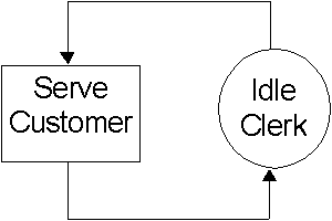
For the customer the cycle is a little more involved because we must arrange for her to appear in the bank and depart from the bank after receiving service. We achieve this by invoking a very general queue known as the 'World Queue' and a special arrival activity.

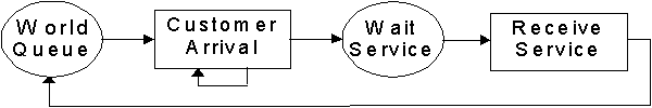
Notice that the customer may pass straight through the 'Wait Service' queue if the Clerk is available to serve him. The arrival activity is rather special as indicated by the sub loop on the symbol. This topic will be taken up further in chapter 3.

All the individual entity cycles are now combined to form a single activity cycle diagram for the model. This is achieved by looking for corresponding activities in the different cycles. In this example the activities 'Receive Service' and 'Serve Customer' are clearly the only common activity. We can now draw the complete Activity Cycle Diagram (ACD).

An activity can only take place if the required quantity of entities is available in each preceding queue. In this example the activity 'Service can only take place if a Clerk is available in the 'Idle Clerk' queue and a Customer in the 'Wait Service' queue.

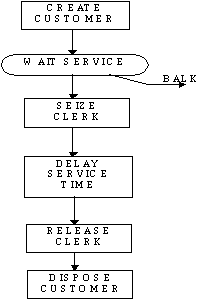The entities again form the focus of the method but they are divided into two classes : Entities proper which move through the model and resources which may be seized and used by the primary entities. In the bank example we can construct the model using the Customer as a primary entity and the Clerk as a resource. Customers are created according to some known arrival distribution and move immediately to the Wait Service queue. Here they will be held until the Clerk is freed by the preceding customer when they, in their turn can seize the Clerk. The 'BALK' is a facility for disposing of customers from the queue when the queue capacity is exceeded. After delaying by their service time the customers release the Clerk to make the Clerk available to any following customers. The Customer entity is finally disposed of. The Process Paradigm is the most intuitive and the one most used by the simulation software available on the market. However the Activity Paradigm has the distinct advantage of providing a completely logical description of the model.

1.5 Maintaining Event Lists

At the heart of Discrete Event Simulation is the concept of an event and the time at which that event occurs. At the outset of the simulation the time at which events will occur (or even the fact that they will occur at all) is unknown apart from the first one or two events. If this were not true there would be no point in carrying out a simulation experiment because all events would be known. This becomes clear when you remember that if the arrival processes and activity times are stochastic then the time spent in a queue by an entity cannot be determined in advance. To progress a simulation through time it is necessary to maintain an ordered list of events and the time at which they are to occur. New events are added to the list as they become known and the current event pointer advances to the next event time on the list. Fig. 1.2 illustrates the idea where successively defined events are labelled E₁, E₂, E₃,…. Etc.

Suppose at time T₁ the event E₅ is about to be processed and that processing E₅ will generate two new events E₉ and E₁₀ at times T₂ and T₃. Fig. 1.2 shows the event list before and after processing E₅

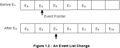
Notice that E9 will occur between E6 and E7 and has been ordered by time of occurrence E10 is presumed to take place after any of the existing events. Once we have established the event list we can process the simulation by a repetition of the following three steps until the simulation is complete :

Start all activities (process all start events) possible at the current simulation time and log any future events that can now be defined. Record any parameters that you wish to keep as the simulation progresses (e.g. the length of queues).

Advance time to the time of occurrence of the next event in the event list.

Stop any activities (process all end events) possible at the current simulation time and move entities onto their next queue.

It is, of course, the job of the simulation language to maintain the event list. to start and stop processes at the appropriate time and record all required statistics. This is a major advantage of using a simulation language over a 3GL for simulation however it is very useful to ensure that you understand the mechanics of the process by trying one or two simulations by hand

The first 10 customers arriving at the bank have their arrival time and service time recorded. Table 1.1 shows the results. Notice immediately that predicting future events by inspection of the table is impossible. For example at what time will the 5^th customer leave the bank ?

Let us use this data to answer the following questions by an event driven hand simulation:

1. What % of time is the clerk idle ?
2. What is the average time a customer spends in the bank ?
3. What is the maximum queue size ?

We start the simulation by drawing up the following event table to record the data and enter the starting conditions.

As soon as we carry out the arrival event at time 3.2 we can predict a departure event for customer 1 at time 3.2 + 3.8 = 7.0 mins. Since the next arrival event is at time 10.9 we know that this departure event will be event number 2 followed by event 3, the arrival of the second customer. Our table now looks like the following :

Notice we can record an idle time figure for the Clerk each time his status changes from idle to busy. After another event our table looks like the following :

You should aim to complete this example by processing all ten customers to answer the problem set.

n

Let us now try an example using the event list in conjunction with the Activity Cycle Paradigm. To follow this example and complete the problem you may find it useful to draw out the ACD on a large sheet of paper and move counters (e.g. small coins) to represent jobs flowing through the system.

A small manufacturing company uses three machines M1, M2 and M3 in its production process. Three products A,B and C are manufactured and each product moves through the machines in the same order M1 - M2 - M3. The process time in hours for each product on each machine is given by the following table

Today the company will manufacture 2 A products, 2 B products and 1 C product. The production manager has decided to manufacture them in the sequence AABBC and needs to know :

1. The queue size before each machine
2. The utilisation of each machine
3. The total production time

It is easy to see that the ACD for this problem is the following :

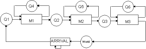
Q1,Q2 and Q3 are the work queues prior to each machine and Q4, Q5 and Q6 are the idle machine queues. We will assume that the arrival activity is defined to allow all jobs to reside in Q1 at time 0.

Start phase : At time 0 we can start the first A product on M1. This allows us to define an end event at time 8 hours when the first A product will finish processing on M1. No other activities can start at time 0

Time phase : Advance time to the next event which is T = 8 when the first A product completes its processing on M1.

End phase : Stop the processing of the A product on M1 and move it to its next queue (Q2). No other activity can end at this time.

Start phase: Start the second A product on M1 and log an end event at time T = 16. Start the first A product on M2 and log an end event at time T = 10. Record the length of the three machine queues.

Time phase: Advance time to the next event (T=10)

The following table reflects the situation at this stage :

When a machine switches from active to idle the active time elapsed since the last period of idleness is recorded and indicated in parenthesise. This enables us to calculate the utilisation of each machine from the definition :

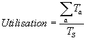
Where T_a is the active time and T_S the total simulation time.

You should complete this simulation