SIMULATION OUTPUT ANALYSIS
Having developed a good simulation model which has been verified and validated. The next step is to perform a series of experiments on the model followed by an analysis of output.
11.1 Introduction
It is not at all uncommon for a simulation user, having spent a considerable amount of time developing a model, to be content with a single run of each experiment and then attempting to interpret the results assuming that a valid set of data has been acquired. That this is wrong is clear when we consider that many of the parameters that describe the model are stochastic and it is not at all surprising that the output shows corresponding stochastic behaviour. A simple example will make this clear.
Example 11.1
Consider a bank containing 4 clerks who serve customers waiting in a single queue. Customers arrive at a rate determined by an exponential inter - arrival time with a mean of 1 minute and all customers have a service time which is also exponentially distributed with a mean of 4 minutes. The bank opens its doors to customers at 9.00 a.m. and closes its doors to new customers at 5.00 p.m. when it completes the days business by servicing the remaining customers in the bank.
This is, of course, an example of an M/M/4 queue and we can theoretically predict that the size of the queue is unstable with these parameters because, with the usual definition ;
![]()
where r is the traffic intensity of the system, l is the arrival rate, m the number of clerks and m the service rate. if r ³ 1 the system shows no long term stability. However for a finite terminating system such as the bank we can run an ARENA model of the system and estimate various output parameters. Table 11.1 shows the results from 10 replications of an ARENA model of this example where a different random number stream has been used for each replication.
Table 11.1 : M/M/4 queue results
|
Replication |
Number served |
End time (hours) |
Aver. time in queue
|
Aver. queue size |
|
1 |
468 |
498.2 |
3.9 |
3.0 |
|
2 |
433 |
494.4 |
2.5 |
1.8 |
|
3 |
472 |
497.4 |
3.3 |
2.6 |
|
4 |
501 |
523.9 |
12.4 |
10.4 |
|
5 |
481 |
528.2 |
21.7 |
17.4 |
|
6 |
461 |
510.9 |
10.3 |
7.9 |
|
7 |
511 |
537.6 |
19.8 |
16.9 |
|
8 |
521 |
498.1 |
4.5 |
3.9 |
|
9 |
500 |
490.1 |
18.0 |
15.0 |
|
10 |
484 |
495.9 |
5.6 |
4.5 |
It is clear from an examination of the table that different replications can result in quite different numbers. This is particularly true if the average queue size is examined which ranges from 1.8 to 17.4 !
Example 11.1 shows us the importance of using valid statistical methods to estimate the expected value of output parameters and to quantify the associated variance.
11.2 Transient and Steady State behaviour
When we start a simulation model running we always start from some initial set of conditions (I). For example implicitly in example 11.1 we assumed a starting condition of no customers in the bank and all four clerks idle. In a manufacturing problem we may start with a particular level of work in progress in the queue for each machine. If Yi is a particular output value at time I of the variable Y then we can define
![]()
The conditional probability P is the probability that the event Yi £ y occurs given the set of initial conditions I. Fi is known as the transient distribution of the variable Y at time i
As the simulation moves away from the initial starting conditions the transient variable evolves (for example its expected value and variance may change, the actual shape of the distribution may change) through a sequence of values F1, F2, F3,....... If this sequence of values approaches a constant value from any initial starting conditions i.e.
![]()
then F(Y) is known as the steady state distribution. The M/M/1 queue shows this behaviour provided that r < 1. Fig. 11.1 shows an ideal variation for the expected value of Yi as a function of I
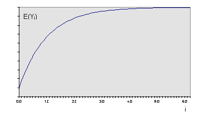
Figure 11.1 : Approach to steady state
| Theoretically the steady state is never reached but (in Fig. 11.1) we might conclude that when I exceeds 4.5 the steady state has effectively been reached. Notice the steady state does not mean that a constant value of Yi has been reached but rather a constant value of E(Yi). The direction and rate of approach to the steady state is also very dependent on the initial conditions as the following result (Fig. 11.2) from Kelton & Law (1985) show. This set of graphs represent an M/M/1 queue with r = 0.9. The parameter s represents the initial number of entities in the queue. | 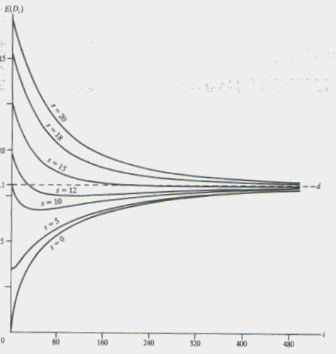
|
We can divide simulation models into two basic types for output analysis :
Two examples of each will make the distinction clear :
Example 11.2 Terminating Systems
A retail or commercial establishment such as a bank or a store opens for business at 9.00 a.m. and closes at 5.00 p.m. On closing no new customers are admitted but existing customers are served before leaving. Initially, of course, the system contains no customers.
A ship yard has obtained an order for 5 bulk carriers which will take in total approximately 2.5 years to complete. The company would like to simulate a range of alternative production plans to minimise on production costs and time. The simulation would start, perhaps, from the date of the last ship of the preceding order leaving the yard.
n
Example 11.3 Non Terminating Systems
In an absolute sense, of course, all systems are terminating since human activity has a finite duration. In terms of simulation modelling we can regard a non terminating system as one in which we wish to model a fixed time duration which forms part of a system which runs for a long time relative to the fixed duration.
As part of a North Sea Oil operation a pipe laying barge is used to continuously lay pipe on the sea bed. The modelling task is to optimise the days throughput of pipe by modelling all the associated activities (including ship delivery of pipe sections, welding sections, coupling sections, painting, X -ray inspection etc.). Clearly examining one days activity is part of a longer process and machines will be either busy or idle at the start and inventory will be at a level determined by the time of the last delivery and the work rate.
A computer network for routing telephone calls from a local area to the wide area network is to be modelled over a 24 hour period. Clearly this is non terminating but it is also different from the previous example in the fact that it is also cyclic because we expect maximum traffic in the morning period, minimum in the middle of the night. It also has a longer periodicity because we can anticipate reduced traffic at week ends.
n
The method of analysis of the two types of system is fundamentally different because for a terminating system we know both the starting conditions and the termination condition. Also if we make replications of the experiment run with differently seeded random numbers we can be sure that the replications are statistically independent.
We will examine terminating systems first and then adapt the analysis to non terminating systems.
11.4 The Analysis of Terminating systems
A terminating system may or may not have a transient period following the start of the simulation. For example the queues which form in a bank may build for half an hour after the doors open and then remain stable (in the sense discussed above) for the remainder of the day. If you are interested in the time an average customer spends waiting in the queue you may wish to exclude this transient period. However in the more usual case the arrival rate of customers varies throughout the day and no initial transient can be recognised and averages are most usefully defined over the whole days trading.
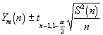
Whatever period is chosen for analysis the basic procedure is the same. The simulation run is replicated n times using a different random number stream in each case to ensure independent trials. If we assume the variation in any output parameter Y is approximately normally distributed we can compute an estimate of the mean using the standard formulae

where the Yi are the means of the individual replications. The sample variance is given by
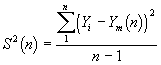
This gives us an approximate 100(1 - a ) percent (0<a <1) confidence interval for the expected value of
Notice that to halve the uncertainty in the mean you need to average four times as many runs.
Example 11.4
For the data in table 5.1 we can estimate the expected average delay in the queue to be given by Ym(10) = 10.2 and the variance S2(10) = 54.48 This gives a variance of the expected value of S2(10)/N = 5.44.
If we accept a confidence level of 90% and apply a 'two tailed' Student's t test to this data we find :
![]()
In other words we have 90% confidence that the expected waiting time in the queue will be 10.2 ± 4.2 minutes.
n
11.4.1 Obtaining a specified precision
In example 11.4 we were able to estimate the precision obtained from replicating the basic experiment 10 times. The value, in that example, turns out to be quite large. The question naturally arises as to how many replications we have to perform to achieve a specified precision ?. Our estimated mean Ym is only an approximation to the true mean (which is unknown) of m . Let us define the absolute error of our estimate as b where
b = |Ym - m |
If we now make replications of our experiment until the half length L1/2 of the 100(1 - a ) percent confidence interval is less than or equal to b then :
In other words Ym has an absolute error of at most b with a probability of 1 - a . Suppose we have constructed a confidence interval for m based on n replications then if we assume that the estimate S2(n) of the population variance will not change appreciably as the number of replications increase an approximate estimate of the number of replications n(b ) required to reduce the absolute error to b or less is given by :
The colon is read as 'such that'.
To find n we can use iteration to increase I by 1 from n until the condition is met.
In practice no simulation results should be quoted or inferences drawn from them unless at least 5 to 9 independent replications have been performed and the variance in the results estimated. Depending on decisions to be made on the basis of the simulation (for example a comparison of two queuing policies) this variance estimate can then be used to decide if further replications are required and if so, how many should be taken.
11.4.2 Limitations
The analysis outlined above assumes that the distributions are normal or near normal in form. If the distributions are seriously skewed (e.g. some Weibull distributions) then calculated confidence intervals may deviate significantly from the calculated (1 - a ) values.
11.5 The Analysis of Non Terminating Systems
In a non terminating system we are usually interested in estimating the steady state values of the output parameters. This assumes that we have successfully identified the transient zone and removed its influence on the analysis. This is difficult to do because the onset of steady state has no precise definition and in general there are no simple rules that can be universally applied to confirm the system is operating in the steady state condition.
Example 11.6 Transients in the M/M/1 queue
The following data was obtained from a simple M/M/1 ARENA simulation with an exponential inter-arrival times with a mean of 22 and an exponential process time with a mean of 20.
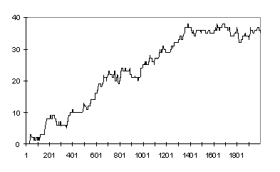
Figure 11.3 : M/M/1 queue to 2000 time units
Over the first 2000 time intervals the data appears to show a classic approach to the steady state. However if we allow the simulation to run for 10,000 time units (Fig. 5.4) we observe that we can no longer make such a simple assumption
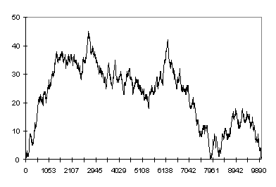
Figure 11.4 : M/M/1 queue to 10,000 time units
Finally if we extend the experimentation out to 500,000 time units we appear to have a very chaotic situation (Fig. 11.5)
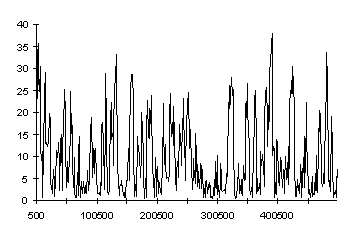
Figure 11.5 : M/M/1 queue to 500,000 time units
n
11.5.1 Using moving averages to estimate the onset of the steady state
At first site it appears that there is no evidence for the onset of steady state conditions in Fig. 11.5 but if we construct a moving average for the results a different picture begins to emerges.
We define the moving average over a window of observations w as follows :
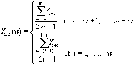
As we increase the size of the window 'w' we average out over a larger range of observations. This has the effect of progressively removing higher frequency components in the output parameter. Fig. 11.6 shows this applied to the data of example 11.6. You can see that if we use a window of w = 101 we are left only with the lowest frequencies.
|
|
In practice because we are interested in defining the onset of the steady state condition we often do not include the calculation of the moving average over the first w observations. This is the approach taken by the MOVAVERAGE command in ARENA (see section 11.6).
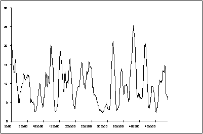
In many cases an even clearer demonstration of the onset of the steady state can be obtained if we compute the cumulative moving average defined as follows :

Fig. 11.7 shows this average applied to the data of example 11.6 and we can now clearly see the onset of steady state behaviour and can predict a mean of 9.6. This agrees very well with the theoretical mean queue size for this M/M/1 queue of
![]()
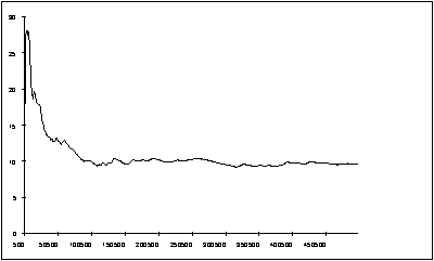
Figure 11.7 : The cumulative mean
11.5.2 Determining the mean and confidence intervals for non terminating systems.
Having identified the steady state region we can now apply the same analysis as used in section 11.4 for terminating systems. To find the confidence interval requires us to replicate the experiment a number of times using different random number streams to ensure independent trials. This procedure is very easy to understand and will give the most reliable results and if computing time and facilities are not limited is probably the best approach to take.
Example 11.7 Estimating the queue size for the M/M/1 queue of example 11.6 (part 1)
From the data graphed in Fig. 11.7 we can conclude that we are in the steady state region beyond a time of 300,000 units. Table 11.2 shows the results of 9 independent replications of the experiment recording the queue size for the data in the steady state region. From this data we can conclude using the equations of section 11.4 that with a confidence level of 90%:
Average queue length : 9.5 ± 1.0
Maximum queue length : 56 ± 6
Table 11.2 : M/M/1 queue results
|
Run num. |
Expected Value |
Max. queue |
| 1 | 11.491 | 75 |
|
2 |
10.840 |
58 |
|
3 |
11.772 |
52 |
|
4 |
8.5289 |
64 |
|
5 |
8.5519 |
48 |
|
6 |
7.3065 |
44 |
|
7 |
8.1125 |
50 |
|
8 |
10.530 |
65 |
|
9 |
8.5477 |
45 |
n
Experiment replication does however have the drawback that for each experiment the transient region has to be passed and its data rejected before the analysis is performed. There have been many proposals for using the data from a single run to estimate the mean and confidence interval to avoid this problem. We will describe two such procedures chosen because facilities exist within ARENA for implementing them.
11.5.3 Using the method of sub intervals (or spectrum analysis)
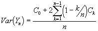
We could avoid the inefficiency of many replications if we could form an estimate of the variance of the mean from a single replication. The problem to be overcome is that near adjacent observations of Y are clearly correlated (e.g. large observations tend to be adjacent to other large observations etc.). We can solve this problem if we can assume that observations are covariance stationary, that is that the covariance between any two observations that are 'k' apart is the same where ever these observations are taken in the sequence. Assuming 'n' observations are left after removing the transient data we compute the sample mean, variance and covariances as follows :
The mean value 
The sample variance 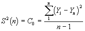
The covariance for a lag of k 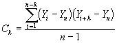
We now estimate the variance in the mean from a weighted sum of all the covariances up to k
To apply the method we need to check the assumption that the observations are covariance stationary. We can achieve this by calculating what is known as the correlation at a lag of k :
![]()
To select a suitable value of k we plot a correlogram which is a plot of mk ~ k. Fig. 11.8 shows an idealised correlogram.
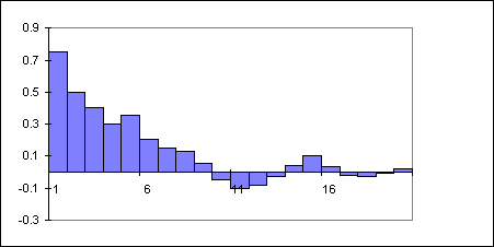
Figure 11.8 : Typical Correlogram
As the correlation values fall to zero we can assume that stationary covariance has been achieved (at approximately 10 in Fig. 11.8).
The main problem with the method is that sample covariance is a biased estimator of the covariance of the mean and thus a large 'n' and a 'k'<<'n' is required to minimise the bias. Generally speaking if k exceeds n/4 the method will probably produce unreliable results.
11.5.4 Batching Observations
Again we take a single replication and discard the observations from the transient region. Now divide the remaining n observations into m batches each of size k (n = mk). If we can assume each batch is equivalent to an independent replication then we can apply the formulae of section 11.4 directly. Now it is clear that the last few observations of batch (k-1) will be correlated with the first few observations of batch k but if the batches are large enough our assumption of independence should be valid. As an estimate of the minimum batch size required we can use the correlogram of the observations and set the minimum batch size to the point where the graph approaches zero. There is no reason why we cannot use batches larger than this minimum provided we retain a total of at least 10 batches to ensure that the Student 't' statistic does not become too large and degrade the confidence half width.
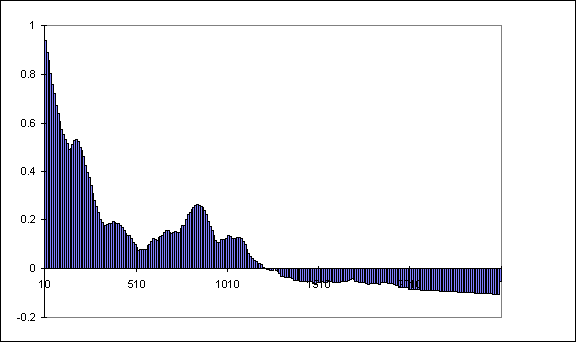
Example 11.7 Estimating the queue size for the M/M/1 queue of example 11.6 (part 2)
Figure 11.9 shows the correlogram for the data from example 11.6 with a lag of 2,500. Provided that we chose a batch size in excess of 1,200 we can expect a reasonable approximation to independent replications. We chose a batch size of 12,000 which gives us 16 batches between a time of 300,000 and 500,000 time units. We can summarise the results as follows :
11.6 ARENA features to support output analysis