A great number of mathematical models of physical systems give rise to differential equations of the type

This is known as Liénard's equation. The system is a generalization of the mass-spring-damper system

previously encountered. In Liénard's equation is the damping term and is the spring term. The equation can be written as the planar system

Under certain conditions on f and g it can be shown that Liénard's equation has a limit cycle. This result is known as Liénard's Theorem.

Theorem - Liénard's Theorem

Suppose that f and g satisfy the conditions
 

(i) f and g are continuously differentiable;

(ii) g is an odd function i.e. ;

(iii) ;

(iv) f is an even function i.e. ;

(v) let and ,

, ();

then Liénard's equation has a unique stable limit cycle surrounding the origin.

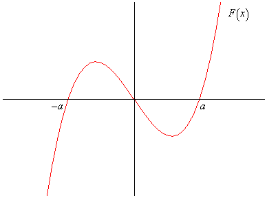
The properties of the odd function F are indicated in the diagram below.

Use the graph to check the properties of F listed above.

• Worked Example 4

where , has a stable limit cycle.

Maple Solution

This is an example of Liénard's equation with

Checking the conditions of Liénard's Theorem we find that
 

(i) both f and g are continuosly differentiable;

(ii)  is odd and obviously ;

(iii)  and so f is even;

(iv) 
 

The conditions are satisfied hence there exists a unique stable limit cycle surrounding the origin.

Van der Pol's equation arose from a 1926 mathematical model of an electrical circuit containing a thermionic valve. Valves were used in early radios and TVs. Careful observation of the damping term shows that for small x the oscillations are negatively damped and hence increase in amplitude. For large x the oscillations are positively damped and hence decrease in amplitude. Intuitively somewhere between these two extremes the damping must be zero resulting in an oscillation with constant amplitude. This is an isolated periodic solution and hence a limit cycle. The most interesting behaviour occurs for relatively large values of the parameter .

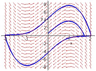
The diagram below shows the phase portrait for the case .

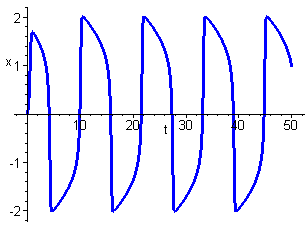
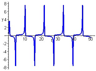
Notice that the limit cycle is very different from one resulting from sinusoidal oscillations. This can be seen clearly in the time series plots of x and y shown below.