4.4.2 Revised model

Essentially, this assumption means that k = b - d varies linearly with the size of the population. The parameter k can be positive or negative depending on the actual population changes taking place. Two possibilities present themselves

and

The assumption k = mP results in the model equation

whose solution is

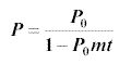
assuming that P = P₀ at t = 0.

Notice that increasing t implies that the value of P approaches zero. This means that our population simply dies out! This is not a very good model since, as the population decreases, the food supply will become adequate because it has to support fewer numbers. Thus the population will tend to increase at some stage not decrease permanently.

The assumption k = mP + c results in the model equation

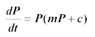
which has two constants.

The model can be developed by considering the value aroond which the population stabilises.

Suppose that the population roughly stabilises at the value P = M

We shall assume that the time derivative of the population is approximately zero when the population reaches rough stability around the value P = M. This gives the equation

so that either

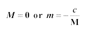
Clearly, the value M = 0 is trivial since we cannot consider a zero population (unless you want to talk about extinct animals!) and so we take .

In this case our model becomes

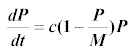
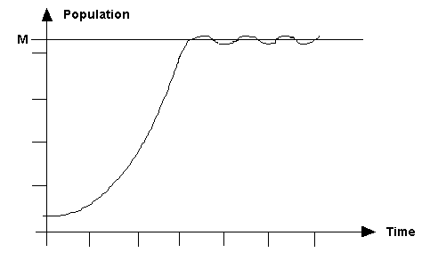
Note that small values of P reduce the equation to which predicts exponential growth for small populations (as expected from the initial model) and that as P approaches M, the maximum value of P, which implies that P remains roughly constant with the variation of time. This equation, which implies exponential growth initially followed by ultimate approximate equilibrium is called the Logistic Equation.