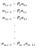
We can now use the above definitions to build the initial model. Firstly, we establish relationships giving us the numbers of females in each age group at time t+1. Take the lowest age group first, the number of members in this group is given by:

The numbers in the remaining classes all follow the same pattern which is given below:

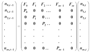
These relationships are best expressed in matrix form as shown below.

A neater way of representing this matrix equation is
nt+1 = Mnt
from which it is clear that
n1 = Mn0
n2 = Mn1 = M2 n0
n3 = Mn2 = M3 n0
.
.
.
so that in general, after p time periods, the population is described by the matrix equation
np = Mpn0
The matrix M is square and of order m+1 and has interesting mathematical
properties which you will be asked to investigate later. In terms of the
modelling process, we need to note that there are m+1 eigenvalues ![]() and corresponding eigenvectors x which satisfy
and corresponding eigenvectors x which satisfy
![]()
and that we can use certain properties of the matrix M and interpret them in terms of a population model.